Showing posts with label Database. Show all posts

Sunday, 26 November 2017

How to connect to postgres RDS from AWS Lambda

Background

In one of the previous post we saw how serverless code works with AWS Lambda and API gateway.
 In this post we will see how we can configure Lambda function to connect to RDS instance and run queries on it. RDS is AWS service for Relational database service. It offers multiple databases like -
  • mysql
  • aurora
  • postgres
  • oracle etc
For this particular post we are going to use  postgres DB. This post is about the lambda function so this assumes you have postgres DB running in RDS and have it's endpoint. username and password handy.

https://www.pgadmin.org/ : If you want a GUI based client to test postgres on local try using pgAdmin.

 How to connect to postgres RDS from AWSa Lambda

Code for Lambda function to connect to RDS is as follows -

'use strict';

const pg = require('pg');
const async = require('async');

const databaseUser = process.env.DB_USER;
const databasePassword = process.env.DB_PASSWORD;
const databaseName = process.env.DB_DB_NAME;
const databaseHost = process.env.DB_HOST;
const databasePort = process.env.DB_PORT;
const databaseMaxCon = process.env.DB_MAX_CONNECTIONS;

exports.handler = (event, context) => {
    console.log('Received event : ' + JSON.stringify(event) + ' at ' + new Date());

    let dbConfig = {
        user: databaseUser,
        password: databasePassword,
        database: databaseName,
        host: databaseHost,
        port: databasePort,
        max: databaseMaxCon
    };

    let pool = new pg.Pool(dbConfig);
    pool.connect(function(err, client, done) {

        if (err) {
            console.error('Error connecting to pg server' + err.stack);
            callback(err);
        } else {
            console.log('Connection established with pg db server');

            client.query("select * from employee", (err, res) => {

                    if (err) {
                        console.error('Error executing query on pg db' + err.stack);
                        callback(err);
                    } else {
                        console.log('Got query results : ' + res.rows.length);
                        
                        
                       async.each(res.rows, function(empRecord) {   
                                console.log(empRecord.name);
                        });
                    }
                    client.release();
                    pool.end();
                    console.log('Ending lambda at ' + new Date());

                });
        }

    });    
    
};

    
}

Explanation 

Here we are using postgres library called pg. You can install this module using -
  • npm install pg

  1. In first part we create a pool of connection giving required parameters to connect to postgres DB. Notice how we are reading these parameters from environment variables. 
  2. Next we call connect on it and pass a callback to get the connection when successful
  3. In the callback we can execute client.query() and pass a callback to get rows of data we need for the employee table.
  4. Finally we iterate over each record using async and print the employee record name.
  5. Release the client when you are done with that particular connection
  6. You can end the pool when all the DB operations are done.


AWS specific notes

  • By default AWS Lambda has internet connection. So it can access web resources.
  • Lambda by default does not have to AWS services running in private subnet.
  • If you want to access services in private subnet eg. RDS running in private subnet then you need to configure the VPC, private subnet to run lambda in and security group is network section of Lambda.
  • However once you do this you will no longer have access to internet (since it is run in private subnet now). 
  • Now if you still need internet access then you need to spin up a NAT gateway or a NAT instance in public subnet and make a route from private subnet to this NAT.
  • Note if you are encrypting lambda environment variable using KMS you will require internet access (KMS needs that). So if your RDS is running in private subnet you need to follow above steps to make it work. Else you are going to get bunch of timeout exceptions.
  • Also note maximum run time of Lambda is 5 mins. So make sure your lambda execution completes withing that time. You should probably limit the queries returned by DB and process that much in one Lambda execution.
  • You can also run lambda as a batch job (using cron expression) from cloud watch.


Related Links

Saturday, 2 September 2017

Understanding database indexes - Part 2

Background

Some time back we took a look at what database indexing is and how it internally works. -
In this post we will see database indexing more from a development design perspective. Many of you might be of the impression that database indexes, tables , performance, lookups maybe responsibility of database admins. Though this might be true to some extent indexes selection, and constructing where clause is developers responsibility and poor choice of indexes and where clause may often lead to performance issues causing queries to run slow. So whenever you are developing an application that requires database interactions as a developer it is very important that you design your indexes first. How do we do that?  - We will see that in sometime. 

Understanding database indexes - Part 2

An index lookup require 3 steps -
  1. B-Tree traversal to root node
  2. Traversal along root node
  3. Access actual table data from each root node
Step 1 is limited is size as tree height/level will be limited by log N constraint. For millions of rows there could be 3-4 level of the tree. It will be extremely rare to see a B-Tree with level more than 5.
You can use following query to see the B-Tree level for your index -

SELECT index_name, blevel+1 FROM user_indexes ORDER BY 2;


blevel gives you the levels of your B-Tree index. Plus one is for the leaf node. So these are the number of levels that needs to be traversed to get an index at the leaf node (considering unique scan).

Step 2 and Step 3 can vary and in most cases are causes of slow index lookup resulting in slow running queries.

Let's start understanding by taking an actual example. Let's create a table as follows -

create table schema8.EMPLOYEE(ID int, name varchar2(255),age int, department varchar2(255), salary int);
alter table schema8.EMPLOYEE ADD CONSTRAINT PRIMARY_KEY PRIMARY KEY (ID); 

CREATE UNIQUE INDEX schema8.UX_EMPLOYEE_1 ON schema8.EMPLOYEE (name, age, department);
ALTER TABLE schema8.EMPLOYEE ADD CONSTRAINT UK_EMPLOYEE_1 UNIQUE (name, age, department) USING INDEX schema8.UX_EMPLOYEE_1;


Lets' add some data in it -

insert into schema8.EMPLOYEE values(1,'Aniket',26,'IT',100);
insert into schema8.EMPLOYEE values(2,'John',29,'FINANCE',40);
insert into schema8.EMPLOYEE values(3,'Sam',27,'IT',101);
insert into schema8.EMPLOYEE values(4,'Ron',30,'ACCOUNTING',35);
insert into schema8.EMPLOYEE values(5,'Sky',33,'DEVOPS',62);
insert into schema8.EMPLOYEE values(6,'Paul',26,'FINANCE',43);
insert into schema8.EMPLOYEE values(7,'Dan',24,'IT',100);
insert into schema8.EMPLOYEE values(8,'Jess',25,'ACCOUNTING',37);
insert into schema8.EMPLOYEE values(9,'Troy',31,'FINANCE',41);
insert into schema8.EMPLOYEE values(10,'Mike',28,'IT',103);
insert into schema8.EMPLOYEE values(11,'Anuj',28,'DEVOPS',64);
insert into schema8.EMPLOYEE values(12,'Vinit',29,'FINANCE',48);
insert into schema8.EMPLOYEE values(13,'Sudhir',29,'ACCOUNTING',39);
insert into schema8.EMPLOYEE values(14,'Anish',28,'IT',100);
insert into schema8.EMPLOYEE values(15,'Shivam',25,'DEVOPS',61);
insert into schema8.EMPLOYEE values(16,'Monica',26,'ACCOUNTING',30);
insert into schema8.EMPLOYEE values(17,'Ramji',32,'FINANCE',41);
insert into schema8.EMPLOYEE values(18,'Anjali',34,'ACCOUNTING',38);
insert into schema8.EMPLOYEE values(19,'Payas',26,'IT',100);
insert into schema8.EMPLOYEE values(20,'Zara',27,'DEVOPS',60);


Normal index


Let's start with a simple query -

select * from schema8.EMPLOYEE where department='IT';


It gives 6 rows. What we really want to understand is the performance of the query and if we can improve it. To understand the queries performance we need to take a look at the execution plan that was used by the sql optimizer. In Sql developer you can just
  • Select the query -> Right click -> Explain -> Explain Plan


And you should see the plan that was selected to run this query and associated cost.

So for above query execution plan is -


As you can see a "FULL TABLE SCAN" was selected.  Since your where clause has department column in it there was no other option. Unique index starting with name could not be used. Primary key index could not be used (Index is always created on primary key -id in this case). So it had to go for a full table scan. Now this is obviously expensive. You can see the cardinality is 6 which basically means there are 6 rows which satisfy "department='IT'" clause and cost is also high.

Let's do something about this. Let's create an index in column department and then again inspect the plan.

create index X_EMPLOYEE_DEPT on schema8.EMPLOYEE(department);


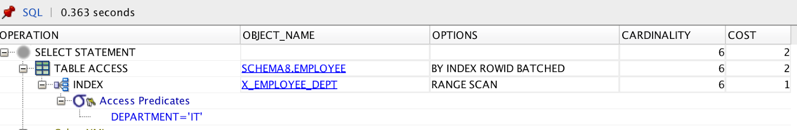
and now lets see the execution plan -


Better? Our cost is reduced by half now. As you can see this time our new index was used for the lookup - "RANGE SCAN". So full table access was avoided. Recall our earlier discussion on steps needed for index lookup -
  1. It used index to get to the leaf node
  2. Traveled along leaf node linked list to find all nodes with department='IT' ("RANGE SCAN")
  3. finally for each index accessed the actual table using rowid to get other table data ("BY INDEX ROWID BATCHED") (Batched because data for all rowids are retrieved in a single call)
Hope this clears how indexes help faster execution of queries.

NOTE :
Cardinality is the estimated number of rows a particular step will return.
Cost is the estimated amount of work the plan will do for that step.
Higer cardinality mean more work which means higher cost associated with that step.
A lower cost query will run faster than a higer cost query.

Primary key index 

As you know primary key has an index created by default. Let's try to query the table using primary key and  see it's execution plan -

select * from schema8.EMPLOYEE where id='12';


As expected cost has further gone down. As primary key index is unique index (since primary key itself is unique) execution plan went for - "UNIQUE SCAN"  and then simple "BY INDEX ROWID" (No batched lookup here since there will be just one entry given that it is unique).  So again if you recollect index lookup steps this consists of -
  1. Use unique index to reach leaf node (Just one leaf node) ("UNIQUE SCAN")
  2. Get the table data ("BY INDEX ROWID")
Notice how there was no traversal among lead nodes and no consequent batch access by row ids.

Unique key index

This would again be same as primary key index since primary key index is also a unique key index but let's give this a try since we have defined unique key for our table on - name, age, department

select * from schema8.EMPLOYEE where name='Aniket' and age=26 and department='IT';

And execution plan for this is -


As expected it is same as primary key index. Instead of primary key index it used unique index we created on our own. Steps are same too.

Composite index

Remember our unique index - name, age, department . We saw in the 1st case where we had department in where clause (before creating an index on department) that this particular index was not used and a full table scan was performed.

If you recollect from our previous discussion index column order matters. If the column order was - department , name, age this new index would gave been picked up. Anyway lets try based on what we already have. Now we are going to add name in where clause and based on our existing knowledge our unique index should get picked up (since it starts with name column) -

select * from schema8.EMPLOYEE where name='Aniket'; 

Execution plan -


As expected our index got used and a full table scan was avoided. However if you use age in where clause index will not be used again - since none of your index starts with age. Try it yourself!

Order of columns in where clause does not matter

We saw how order of columns matter in index creation. Same does not apply for where clause column order. Eg consider -

select * from schema8.EMPLOYEE where name='Aniket' and age=26;
select * from schema8.EMPLOYEE where age=26 and name='Aniket';


SQL optimizer is intelligent enough to figure out name is one of the column in where clause and it has an index on it that can be used for lookup and it does so -

For each query above execution plan is -


And that concludes  - order of columns in where clause does not matter!

Multiple indexes applicable - select the one with least cost

So far we have seen various cases in which just one index was applicable. What if there are 2. Let's say you use department and name in your where clause. Now there are 2 options -
  1. Use the unique index starting with name 
  2. Use the index in department
Let's see how it works out -

select * from schema8.EMPLOYEE where name='Aniket' and department='IT';


Execution plan -


As you can see index on name was selected and once leaf nodes were retrieved filter was applied in it to get those rows with department='IT' and finally batched rowid access to get all the table data. This index was selected probably because unique indexes are given preference over non unique index since they are faster. But it depends totally on sql optimizer to figure that out based on execution cost.

Covered indexes and queries

In our previous discussion we saw what covered indexes/queries are. They are basically indexes that have all the data needed to be retrieved and there is no need to access the actual table by rowid. FOr eg. consider -

select name, age,department from schema8.EMPLOYEE where name='Aniket';

Take some time to think this though based on our discussion so far. We know where clause has name it it. We also know we have an unique index that starts with name. So it will be used. On top of that we have an added bonus - we just need name,age,department that us already part of that unique index. So we really don't need to access to actual table data to get any other content.

Let's see this execution plan -


 As expected. There is no "BY INDEX ROWID" or "BY INDEX ROWID BATCHED". That's because table access is not needed since all required data is in index itself. Also note the range scan - even though unique index is used there is no unique row returned since only part of unique index is used.

Summing Up

So to sum up execution plan can do -
  • FULL TABLE SCAN or
  • UNIQUE SCAN or
  • RANGE SCAN
 and then access the table data (if needed) with -
  • BY INDEX ROWID or
  • BY INDEX ROWID BATCHED
Either case you need to choose index very wisely based on your where clause, it's combination. Order of columns in index is very important. Always go for index that starts with column that is used in most of the queries where clause. Also go for equality first than range. So if you where clause is something like - "where name='Aniket' and age>24" always for name as column ordered before age. since equality will give less results to filter from. Age will be applied as filter in above case.

Related Links

Sunday, 27 August 2017

Understanding having clause in SQL

Background

If you have written queries or worked on a project that requires database support then you must have use or atleast familiar with having clause. This is also one of the popular interview questions for beginners to test database knowledge if you ask me. Simple syntax looks like -


SELECT column_name(s)
FROM table_name
WHERE condition
GROUP BY column_name(s)
HAVING condition
ORDER BY column_name(s);


So your 1st and foremost answer is that you use having clause with "group by" clause. How and why we will come to later part in of this discussion. Having said that before we proceed make sure you know what group by clause does. Also you need to have an idea of what aggregate functions are . Eg. min(), max(), count(), sum() etc.


Understanding having clause in SQL

So far we know we use having clause with group by clause. Let's answer the question why. 

Let's say you have a table employee which have basic data of an employee - id, name, department etc. 

Problem statement : Now we are interested to find out how many employees are there in each department and probably see the result in sorted order so that department with maximum employees is displayed first. How would you do this? Using following query -

select department, count(*) from employee group by department order by count(*) desc;

This works fine.  Now let's redefine our problem statement.

Problem statement :  Let's say we now want the same thing - department and number of employees in each department sorted in descending order. However this time we have an additional constraint. We want to see only those departments that have more than 10 employees in it. You would probably try -

select department, count(*) from employee group by department where count(*) > 10 order by count(*) desc;

Problem : Does not work
Error : ORA-00934: group function is not allowed here
             00934. 00000 -  "group function is not allowed here"
(Above error is show for oracle database)

NOTE :  An aggregate may not appear in the WHERE clause unless it is in a subquery contained in a HAVING clause or a select list, and the column being aggregated is an outer reference

Problem is that you cannot use aggregate functions in where clause. Solution? - Having clause. This is exactly why having clause was introduced. Once you have applied the group by clause and wish to filter the data further on the results obtained you use having clause. So your correct query would be -


select department, count(*) from employee group by department having count(*) > 10 order by count(*) desc;

Aggregate functions are allowed in having clause. So lets go over the original syntax again and see how it works -

SELECT column_name(s)
FROM table_name
WHERE condition
GROUP BY column_name(s)
HAVING condition
ORDER BY column_name(s);

  1. First you select  column_name(s) from the table that match the where clause condition
  2. Once result is obtained then group by clause is applied to it to get the next set of result.
  3. Once that is done condition is having clause is applied to further filter the result.
  4. Finally order by clause is applied to sort the result as required and return.

NOTE :  where clause us applied to filter results before group by clause is applied where as having clause is applied after.

Other alternative can be like -

select department, count from ( 
select department, count(*) count from employee group by department )\
where  count>10;

Related Links

Saturday, 5 August 2017

Select top N records from each category in PL/SQL

Background

Lets say you have 2 tables -
  1. EMPLOYEE
  2. EMPLOYEE_SALARY
EMPLOYEE table has employee id which is a primary key and his name.  EMPLOYEE_SALARY has employee id which is foreign key to id in EMPLOYEE table. This table has employee department and salary. You need to write a query that returns top 2 employees from each department that has highest salary.

Tables creation and data insertion

Table Queries :

create table schema8.EMPLOYEE(ID int, name varchar2(255));
alter table schema8.EMPLOYEE ADD CONSTRAINT PRIMARY_KEY PRIMARY KEY (ID);
create table schema8.EMPLOYEE_SALARY(EMPLOYEE_ID int, department varchar2(255), salary int);
alter table schema8.EMPLOYEE_SALARY ADD CONSTRAINT FK_EMP_ID FOREIGN KEY (EMPLOYEE_ID) REFERENCES schema8.EMPLOYEE(ID);

Data Queries for  EMPLOYEE table:

insert into schema8.EMPLOYEE values(1,'Aniket');
insert into schema8.EMPLOYEE values(2,'John');
insert into schema8.EMPLOYEE values(3,'Sam');
insert into schema8.EMPLOYEE values(4,'Ron');
insert into schema8.EMPLOYEE values(5,'Sky');
insert into schema8.EMPLOYEE values(6,'Paul');
insert into schema8.EMPLOYEE values(7,'Dan');
insert into schema8.EMPLOYEE values(8,'Jess');
insert into schema8.EMPLOYEE values(9,'Troy');
insert into schema8.EMPLOYEE values(10,'Mike');

 Data Queries for EMPLOYEE_SALARY table:

insert into schema8.EMPLOYEE_SALARY values(1,'IT',10000);
insert into schema8.EMPLOYEE_SALARY values(2,'Admin',500);
insert into schema8.EMPLOYEE_SALARY values(3,'Sales',1200);
insert into schema8.EMPLOYEE_SALARY values(4,'Sales',1500);
insert into schema8.EMPLOYEE_SALARY values(5,'IT',9000);
insert into schema8.EMPLOYEE_SALARY values(6,'Admin',4000);
insert into schema8.EMPLOYEE_SALARY values(7,'Admin',5000);
insert into schema8.EMPLOYEE_SALARY values(8,'IT',9500);
insert into schema8.EMPLOYEE_SALARY values(9,'Sales',1000);
insert into schema8.EMPLOYEE_SALARY values(10,'Admin',6000);

Final data :
select * from schema8.EMPLOYEE;
select * from schema8.EMPLOYEE_SALARY;


Solution

We are going to use RANK to partition by department and order by salary - 

select * from (
select id , name, department, salary, RANK() over (partition by department order by salary desc) as rank from(
select e.id, e.name, es.department,es.salary from schema8.EMPLOYEE e left OUTER join schema8.EMPLOYEE_SALARY es on (e.id=es.employee_id))
) where rank <= 2;


First we have done a left outer join so that we capture all employee records with their respective salaries and departments. In outer query we have ranked it based on their salaries in respective department. Finally we select all records that have rank <=2 i.e top 2 records.


Related Links


Monday, 31 July 2017

Install Oracle instant client and sqlplus using Homebrew

Background

 In one of the previous posts we say how to install and run sql plus  and Oracle instant client  on Ubuntu operating system -
In this post we will see the same for a Mac.

This post expects you have homebrew installed. If not please refer -

 Install Oracle instant client and sqlplus using Homebrew

For this you need to download following two files -
  1. instantclient-basic-macos.x64-12.1.0.2.0.zip 
  2. instantclient-sqlplus-macos.x64-12.1.0.2.0.zip 
You can download these files from oracle site - http://www.oracle.com/technetwork/topics/intel-macsoft-096467.html

Once download copy these files into following folder-
  •  ~/Library/Caches/Homebrew 
 Once done run following commands -
  • brew tap InstantClientTap/instantclient
  • brew install instantclient-basic
  • brew install instantclient-sqlplus
 This should install sqlplus for you.


Related Links

Monday, 15 May 2017

How does database indexing work?

Background

Database indexing is a wide topic. Database indexing plays a important role in your query result performance. But like everything this too has a trade off.  In this post we will see what database indexing is and how does it work.


Clustered and Non clustered index

Before we go to how indexing actually works lets see the two types on indexes -
  1. Clustered index
  2. Non clustered index
Data in tables of a database need to be stored on a physical disk at the end of the day. It is important the way data is stored since data lookup is based on it. The way data is stored on physical disk is decided by an index which is known as Clustered index. Since data is physically stored only once , only one clustered index is possible for a DB table. Generally that's the primary key of the table. That's right. Primary key of your table is a Clustered index by default and data is stored physically based on it.

NOTE : You can change this though. You can create a primary key that is not clustered index but a non clustered one. However you need to define one clustered index for your table since physical storage order depends on it.

Non clustered indexes are normal indexes. They order the data based on the column we have created non clustered index on. Note since data is stored only once on the disk and there is just one column(or group of columns ) which can be used to order stored data on disk we cannot store the same data with ordering specified by non clustered index (that's the job of clustered index). So new memory is allocated for non clustered indexes. These have the column on which it is created as the key of the data row and a pointer to the actual data row (which is ordered by clustered index - usually the primary key). So if a search is performed on this table based on the columns that have non clustered indexes then this new data set is searched (which is faster since records are ordered with respect to this column) and then the pointer in it is used to access the actual data record with all columns.


Now that we have knowledge of clustered and non clustered indexes lets see how it actually works.

Why is indexing needed?

When data is stored on disk based storage devices, it is stored as blocks of data. These blocks are accessed in their entirety, making them the atomic disk access operation. Disk blocks are structured in much the same way as linked lists; both contain a section for data, a pointer to the location of the next node (or block), and both need not be stored contiguously.

Due to the fact that a number of records can only be sorted on one field, we can state that searching on a field that isn’t sorted requires a Linear Search which requires N/2 block accesses (on average), where N is the number of blocks that the table spans. If that field is a non-key field (i.e. doesn’t contain unique entries) then the entire table space must be searched at N block accesses.

Whereas with a sorted field, a Binary Search may be used, this has log2 N block accesses. Also since the data is sorted given a non-key field, the rest of the table doesn’t need to be searched for duplicate values, once a higher value is found. Thus the performance increase is substantial.

What is indexing?

This is rather a silly question given we already saw clustered and non clustered indexes but lets give it a try.

Indexing is a way of sorting a number of records on multiple fields. Creating an index on a field in a table creates another data structure which holds the field value, and pointer to the record it relates to. This index structure is then sorted, allowing Binary Searches to be performed on it. This index is obviously the non clustered one. There is no need to create separate data structure for Clustered indexes since the original data is stored physically sorted based on it.

The downside to (non clustered) indexing is that these indexes require additional space on the disk, since the indexes are stored together in a table using the MyISAM engine, this file can quickly reach the size limits of the underlying file system if many fields within the same table are indexed.

Performance

Indexes don't come free.  They have their own overhead. Each index creates an new data set ordered by the columns on which it is created. This takes extra space (though not as much as the original data set since this just has single data and pointer to actual row data). Also inserts are slower now since each insert will have to update this new index data set as well. Same goes for deletion.

Data structures used in indexes

Hash index :
 Think of this using a HashMap. Key here would be derived from columns that are used to create a index (non clustered index to be precise). Value would be pointer to the actual table row entry. They are good for equality lookups like get rows of data of all customer whose age is 24. But what happens when we need a query like set of data of customer with age greater than 24. Hash index does not work so go in this case.  Hash indexes are just good for equality lookups.
Eg.


B-tree Indexes:
These are most common types of indexes. It's kind of self balancing tree. It stores data in an ordered manner so that retrievals are fast. These are useful since they provide insertion, search and deletion in logarithmic time.
Eg.


Consider above picture. If we need rows with data less that 100 all we need are notes to the left of 100.

These are just common ones. Others are R-tree indexes, bitmap indexes etc.

 To get a complete idea on how indexes work internally please refer - SQL Indexing and Tuning.

NOTE : There is no clustered index in oracle database. A regular non clustered is automatically created on primary key. As an alternative in Oracle DB you can explore Index organized tables.


Important Points to remember

  • Avoid using function in where clause which takes column parameter as index. Functions render indexes useless. Functions are like blackbox and database optimized does not know about it's relationship with argument the function takes. So instead of using the index it will perform full table scan. Eg
    • create index employee_name_idx on employee(name);
    • select * from employee where name='Aniket'; --uses index
    • select * from employee where lower(name)='aniket'; --cannot use index
  •  If you do have a concatenated index then choose the column order so that mulitple sql queries (of you usecases) can use it. Eg.
    • select * from employee where name='Aniket'; --sql1
    • select * from employee where name='Aniket' and age=26; -- sql2
    • create index employee_name_idx on employee(name, age);  --correct
    •  create index employee_name_idx on employee(age, name);  --incorrect (sql1 cannot use this)
  • Avoid like expressions in your where clause which starts with a wildcard. it will be of no use even the column is indexed. Eg.
    • create index employee_name_idx on employee(name);
    •  select * from employee where name like '%ket'; -- will be very slow
    •  select * from employee where name like 'Anik%'; --will be fast as it used prefix on index
  • Always index for equality first (vrs lets say a range)
    •  create index employee_name_idx1 on employee(joining_date, name);  --slower
    •  create index employee_name_idx2 on employee( name, joining_date); --faster
    • select * from employee where name='Aniket' and  joining_date >= TO_DATE('2017-08-20')
  • Always check if covered indexes are possible. This prevents actual table access since you get all the data in index only. So lets say you have a table with columns A-Z. Also lets say you have an index on column B and your query is something like -
    • select A from table where B='XYZ'
    • Query looks good and it will use our index defined on column B and speed up the query time in the process but for each hit in btree leaf of index it will need to access actual table row to get A.
    • Now consider you have index on (B,A). Since your where clause has B this index will be picked up. However in this case once entries are located we already have value of A which we need to find. So this will avoid lookup of actual table row.
    •  This obviously depends on your use case. None the less it's important to consider this use case.

Related Links

Sunday, 12 February 2017

Understanding JDBC and building database applications with it

Background

JDBC stands for Java database connectivity. This includes connecting to DB in Java, running queries and processing results.

A relational DB that has tables consisting of rows and columns. You can interact with a relational DB with -
  • JDBC APIs. You get a connection, create a statement and get result set of the query.
  • Use JPA(Java persistence API). This uses a concept called ORM (Object relational mapping) where you map Java objects to tables and operate on these objects. For eg. hibernate is one such framework.
  • SQL (Structured query language) is used to interact with the relational DB. 
 In this post we are going to understand JDBC.

Interfaces in JDBC

All JDBC classes in Java are part of java.sql.* package.  There are 4 important interfaces that you need to understand -
  1. Driver : Know how to get connection from DB
  2. Connection : Knows how to interact with DB
  3. Statement : Knows how to run SQL on the DB
  4. ResultSet : Knows the result returned by the SQL query from the DB.
 To see a sample Java code on how to connect to a DB from Java you can see one of my previous posts -
Above code snippet uses mysql DB but you can use any DB really. There are some common things that we sill see in a moment.

NOTE : You no longer have to explicitly load the driver class using Class.ForName(driver). From JDBC 4 driver class is automatically loaded from the class path. 

Building DB application with JDBC

Let's start by looking at how JDBC url looks like and is constructed -


 As you can see JDBC URL is split into 3 parts -
  1. 1st part is the jdbc protocol
  2. 2nd part is the name of the DB. For eg. mysql, postgres, derby or oracle
  3. 3rd part is respective DB specific format
You have already seem mysql connection string in code above -
  • jdbc:mysql://localhost:3306/testDB
 Some other examples are -
  • jdbc:postgresql://localhost/testDB
  • jdbc:oracle:thin:@192.168.1.45:1699:testDB
  • jdbc:derby:testDB
 Once you know the URL first step is to load the DB specific driver. As mentioned before traditionally you needed to explicitly load the driver using -
  • Class.ForName(driver)
But since JDBC 4 you don't. Java loads automatically for you if it's present in the classpath.  Once driver is loaded next you need to get the Connection from it. You can do so with -
  • Connection conn = DriverManager.getConnection("jdbc:derby:testDB");
 NOTE : If you get exception like "java.sql.SQLException: No suitable driver found for..." then the driver is not present on the classpath. Add it.

Once you have the connection you can get the Statement from it as follows -
  • Statement stmt = conn.createStatement();
  Once you have the statement you are all set to execute queries on DB -
  • ResultSet rs = stmt.executeQuery("select * from countries");
  • int res = stmt.executeUpdate("insert into countries values(1, 'India')");
 NOTE : ResultSet points to a location before 1st row when it is result. To access the data you need to call rs.next() which returns a boolean stating if more result is present. If it does you can access it via rs.getInt(1) etc.

NOTE : Column indexes start with 1. So something like rs.getInt(0)will throw SQL exception.

Once you have processed the result set never forget to close the resources and that include your -
  • ResultSet
  • Statement
  • Connection
NOTE : It is very important to close resources in the right order. If you don't want to close it manually you can always use it under try with resource statements so that Java closes them for you. If doing manually you can close it in finally statement with null checks.


Why do we use a DataSource instead of a DriverManager?

 Always use a datasource over DriverManager as-


  • Client app need not know about the DB details, username , password. App server will take care of it. With datasource all you need is a jndi name properties of which can be configured at app level.
  • App server takes care of creating and closing connections. You don’t have to manage it in your client application.
  • Data source has support for creating pool of connection whereas data manager does not.


  •  Why do we use a PreparedStatement instead of a Statement

    You should always use PreparedStatement instead of a Statement. PreparedStatement is subclass of Statement. This has multiple reasons -
    • Performance: A PreparedStatement figures out a plan to run the SQL and remembers it. Helps when same query is run multiple times.
      • Databases like sql server or oracle databases  have execution plan cache. They can resue the execution plan while running the same query again. This saved efforts in rebuilding execution plan. However this will work only when the sql query is exactly the same. If it has different values than db treats it as different query. In case of Prepared statements in which we use bind parameters we use placeholders so that the query remains the same and subsequently the execution plan. Bind parameters are hidden to the database query optimizer.
    • Security: To prevent SQL injection. It's a famous hacking technique. Go ahead read it up on google.
    • Readability: No String concatenations in building queries.

    Related Links

    Thursday, 18 August 2016

    Installing MongoDB in Mac

    Background

    Sometime back I had written a post on MongoDB. Installation and basic syntax in Windows - Getting Started with MongoDB . This post is starting of series of posts on MongoDB. In this post we will see installation and configuration of MongoDB in Mac.

    Installing MongoDB

    • Go to MongoDb download center and download the tgz of the latest build. Your OS should already be selected and you should see the download link.
    • You can also install MongoDB using homebrew
      • brew install mongodb  (To install the MongoDB binaries)
      • brew install mongodb --with-openssl (To install the MongoDB Binaries with TLS/SSL Support)
      • brew install mongodb --devel  (To install the latest development release)
    • Once you have downloaded that tarball you can unpack it using following command - 
      • tar xvf mongodb-osx-ssl-x86_64-3.2.9.tgz
    • Once you have unpacked it navigate to that folder and then into bin folder inside it. Here you will see list of programs. There are two programs here of out interest - 
      • mongo : This is the mongo shell used to connect to the mongo DB.
      • mongod : This is the actual server.
    • That's it your mongo db is installed and ready to be run.
    NOTE : MongoDB by default stores its data in directory "/data/db". So make sure this directory is created with necessary permissions. 
    • sudo mkdir -p /data/db
    • sudo chmod -R 777 /data/

    If you want to give a custom path you can give it when you start mongodb - 
      --dbpath arg                          directory for datafiles - defaults to "/data/db"
    Eg.
    • mongod --dbpath /data/mydb

    Running and connecting MongoDB

    • To run MongoDB server go to bin directory and start mongod program.
      • ./mongod
    • This should start your mongodb server listening on default port 27017.
    • To see all mongod configuration options you can type - 
      • ./mongod --help


    Once mongodb is up you can try connecting to it using mongo shell.
    You can start mongo shell by
    • ./mongo
    You can also see incoming connection in your server console -
    • 2016-08-18T22:34:27.315+0530 I NETWORK  [initandlisten] connection accepted from 127.0.0.1:56356 #1 (1 connection now open)
       
    Once you are connected you can try following operations - 
    • use mydb
    • db
    • show dbs
    • db.testCollection.insert({"Name":"John"})
    • show collections
    • db.testCollection.find()
     That's it for the basic of installing Mongo DB on your Mac. To avoid always going till bin to execute your programs you can do either of of the follwing -
    1. Add you path to bin to your PATH and export it. OR
    2. Add all these binaries to /usr/local/bin/ by
      • cp * /usr/local/bin
    3. You can verify it by wither running - 
      1. which mongod OR
      2. mongod --help

    Related Links

    Thursday, 9 June 2016

    Remove duplicate rows from table in Oracle

    Background

    This is classic database question to check candidates knowledge about SQL queries. You have a table where lets say you have duplicate entries (lets also say column1 and column2 can form a candidate key). Now you need to remove duplicates from then table. That is all rows in the table should be distinct. How would you do this?

     Query to remove duplicate rows from table in Oracle

    You can execute following query to remove duplicates - 

    DELETE FROM your_table
    WHERE rowid not in
    (SELECT MIN(rowid)
    FROM your_table
    GROUP BY column1, column2);
    

    column 1 and column2 as I mentioned for candidate keys. You can very well add all columns in it.

    Example

    Queries :
    create table schema8.EMPLOYEE(ID int, name varchar2(255));
    insert into schema8.EMPLOYEE values(1,'Aniket');
    insert into schema8.EMPLOYEE values(1,'Aniket');
    insert into schema8.EMPLOYEE values(1,'Aniket');
    insert into schema8.EMPLOYEE values(2,'John');
    insert into schema8.EMPLOYEE values(2,'John');
    insert into schema8.EMPLOYEE values(3,'Sam');
    insert into schema8.EMPLOYEE values(3,'Sam');
    insert into schema8.EMPLOYEE values(3,'Sam');


    ROWID Pseudocolumn  in Oracle

    For each row in the database, the ROWID pseudocolumn returns the address of the row. Oracle Database rowid values contain information necessary to locate a row.

    Rowid values have several important uses:
    • They are the fastest way to access a single row.
    • They can show you how the rows in a table are stored.
    • They are unique identifiers for rows in a table.
    NOTE : You should not use ROWID as the primary key of a table. If you delete and reinsert a row with the Import and Export utilities, for example, then its rowid may change. If you delete a row, then Oracle may reassign its rowid to a new row inserted later.

    NOTE : Although you can use the ROWID pseudocolumn in the SELECT and WHERE clause of a query, these pseudocolumn values are not actually stored in the database. You cannot insert, update, or delete a value of the ROWID pseudocolumn.

    Related Links

    Saturday, 4 June 2016

    Simple PL/SQL code to throw NO_DATA_FOUND exception

    Background

    Good database question for beginners.Write a simple PL/SQL code snippet to throw NO_DATA_FOUND exception. You cannot raise this exception. Maybe try to understand how the candidate answers this. Simple code is as follows - 

    DECLARE
       nowt VARCHAR(10);
    BEGIN
       SELECT * INTO nowt FROM DUAL WHERE 1=0;
    END;
    /
    

    and it should throw the exception - 

    Error starting at line 8 in command:
    DECLARE
       nowt VARCHAR(10);
    BEGIN
       SELECT * INTO nowt FROM DUAL WHERE 1=0;
    END;
    Error report:
    ORA-01403: no data found
    ORA-06512: at line 4
    01403. 00000 -  "no data found"
    *Cause:    
    *Action: 


    Related Links

    Saturday, 14 May 2016

    Redis Tutorial (Basics & Configuration)

    Background

    I am just going to quote Redis from their website -

    "Redis is an open source (BSD licensed), in-memory data structure store, used as database, cache and message broker. It supports data structures such as strings, hashes, lists, sets, sorted sets with range queries, bitmaps, hyperloglogs and geospatial indexes with radius queries. Redis has built-in replication, Lua scripting, LRU eviction, transactions and different levels of on-disk persistence, and provides high availability via Redis Sentinel and automatic partitioning with Redis Cluster."

    It is written in C language.


    Peculiar features /  Advantages

    • Very Fast : Since Redis stores it's data entirely in memory (used disk for persistence) it is very fast in terms of I/O.
    • Various Data Structure Support : As saw before it supports data structures such as strings, hashes, lists, sets, sorted sets with range queries, bitmaps, hyperloglogs and geospatial indexes with radius queries.
    • Atomic operations : All Redis operation are atomic which means there is no race condition. Each client/thread will get updates data.
    • Multi Usability - Redis can be used as a database, as a cache or a message broker (like activeMQ)

    Installation

    To install redis simply install following command -
    • sudo apt-get install redis-server

    To start redis server run following command
    • redis-server


    That's it your redis server is up and running.

    You can test your server with redis-cli
    • redis-cli
    and then type ping you should get reply as pong


    NOTE : You can also install redis desktop manager for Ubuntu

    You can set the redis configuration using following command -
    • CONFIG GET CONFIG_SETTING_NAME
    You can get all configuration by using *
    •  CONFIG GET *
    To edit a configuration use following command -
    • CONFIG SET CONFIG_SETTING_NAME VALUE


     Data Types in Redis

    There are 5 data types that redis supports -
    1. Strings
    2. Hashes
    3. Lists
    4. Sets
    5. Sorted Sets

     Strings

    You can do string data storage with GET and SET commands. You can store upto 512 MB of data in a String.
    • SET name aniket
    • get name

     Hashes

    Sets the specified fields to their respective values in the hash stored at key. This command overwrites any existing fields in the hash. If key does not exist, a new key holding a hash is created.

    You can do hash operations with HMSET, HGET or HGETALL
    •  HMSET employee1 name aniket code 007
    •  HGET employee1 name
    •  HGETALL employee1


    Lists

     Insertion order is retained. You can use lpush and lrange to add and view the list
    • lpush countrylist India
    • lpush countrylist China
    • lrange countries 0 -1


    Sets and Sorted Sets

    Sets are unorderd collection of strings where as in sorted setseach string is associated with a score that is used to sort the strings.

    You can use SADD and SMEMBERS to add and view members of a set where as you can use ZADD and ZRANGEBYSCORE to add and view strings in sorted sets.

    In sets each string is unique unlike list. So adding same key twice will result in just one entry in the set.


    Related Links


    Friday, 13 May 2016

    Hibernate tutorial with xml configurations

    Background

    Hibernate is Java ORM (Object relation mapping) tool. It like other ORMs help map Java domain objects with tables in relational databases. It removes the overhead of using the underlying JDBC calls. It supports CRUD operations across all major relational databases. It supports transaction management and many other features. In this post we will see a demo example of hibernate application.


    Architecture


    Setup

    I am simply going to create a simple standalone Java application using hibernate that used oracle database to connect to.  Also I am using Eclipse IDE with Apache Ivy dependency management tool. So create a project called HibernateDemo. It's structure will be as follows - 


    Next lets create required files one by one. Lets start with the table creation. Following SQL should create the desired table for us in oracle - 

     CREATE TABLE Employee (
    
      id number(10) NOT NULL PRIMARY KEY,
    
      name varchar2(20) DEFAULT NULL,
    
      gender varchar2(20) DEFAULT NULL,
    
      accesstime_time DATE DEFAULT (sysdate)
    
    );
    

     Next you will need some dependency jars like hibernate, slf4j etc. Add following dependency in ivy file - 

    <?xml version="1.0" encoding="ISO-8859-1"?>
    <!--
       Licensed to the Apache Software Foundation (ASF) under one
       or more contributor license agreements.  See the NOTICE file
       distributed with this work for additional information
       regarding copyright ownership.  The ASF licenses this file
       to you under the Apache License, Version 2.0 (the
       "License"); you may not use this file except in compliance
       with the License.  You may obtain a copy of the License at
    
         http://www.apache.org/licenses/LICENSE-2.0
    
       Unless required by applicable law or agreed to in writing,
       software distributed under the License is distributed on an
       "AS IS" BASIS, WITHOUT WARRANTIES OR CONDITIONS OF ANY
       KIND, either express or implied.  See the License for the
       specific language governing permissions and limitations
       under the License.    
    -->
    <ivy-module version="2.0" xmlns:xsi="http://www.w3.org/2001/XMLSchema-instance"
           xsi:noNamespaceSchemaLocation="http://ant.apache.org/ivy/schemas/ivy.xsd">
        <info
            organisation="ofsg.com"
            module=""
            status="integration">
        </info>
        
        <dependencies>
            <dependency org="org.hibernate" name="hibernate-core" rev="5.1.0.Final"/>
            <dependency org="org.slf4j" name="slf4j-simple" rev="1.7.21"/>
        </dependencies>
        
        
    </ivy-module>
    

    You will also need to manually add oracle OJDBC jar in the classpath.

    Java Code and configurations


    Next lets create our persistent Java class - Employee.java


    package com.osfg.models;
    
    
    import java.util.Date;
    
    /**
     * 
     * @author athakur
     * 
     */
    public class Employee {
    
        private int id;
        private String name;
        private String gender;
        private Date accessTime;
    
        public int getId() {
            return id;
        }
    
        public void setId(int id) {
            this.id = id;
        }
    
        public String getName() {
            return name;
        }
    
        public void setName(String name) {
            this.name = name;
        }
    
        public String getGender() {
            return gender;
        }
    
        public void setGender(String gender) {
            this.gender = gender;
        }
    
        public Date getAccessTime() {
            return accessTime;
        }
    
        public void setAccessTime(Date accessTime) {
            this.accessTime = accessTime;
        }
    
    }


    Next lets create configuration files that map this class to the database table - employee.hbm.xml

    <?xml version="1.0"?>
    <!DOCTYPE hibernate-mapping PUBLIC "-//Hibernate/Hibernate Mapping DTD 3.0//EN"
    "http://hibernate.org/dtd/hibernate-mapping-3.0.dtd">
    
    <hibernate-mapping>
        <class name="com.osfg.models.Employee" table="EMPLOYEE">
            <id name="id" type="int">
                <column name="ID" />
                <generator class="assigned" />
            </id>
            <property name="name" type="java.lang.String">
                <column name="NAME" />
            </property>
            <property name="gender" type="java.lang.String">
                <column name="GENDER" />
            </property>
            <property name="accessTime" type="timestamp">
                <column name="ACCESS_TIME" />
            </property>
        </class>
    </hibernate-mapping>


    NOTE : Notice the generator class. It is set to assigned so that you manually assign the primary key. There are many generator classes such as assigned (It is used if id is specified by the user), increment, hilo, sequence, native etc.

    Now lets see the hibernate configuration file that has database connection details - hibernate.cfg.xml

    <?xml version='1.0' encoding='UTF-8'?>  
    <!DOCTYPE hibernate-configuration PUBLIC  
      "-//Hibernate/Hibernate Configuration DTD 3.0//EN"  
      "http://hibernate.sourceforge.net/hibernate-configuration-3.0.dtd">  
      
    <hibernate-configuration>  
      
    <session-factory>  
    <property name="hbm2ddl.auto">update</property>  
    <property name="dialect">org.hibernate.dialect.Oracle10gDialect</property>  
    <property name="connection.url">jdbc:oracle:thin:@localhost:1699/test</property>  
    <property name="connection.username">system</property>  
    <property name="connection.password">test</property>  
    <property name="connection.driver_class">oracle.jdbc.driver.OracleDriver</property>  
    <mapping resource="/com/osfg/resources/employee.hbm.xml"/>  
    </session-factory>  
      
    </hibernate-configuration>  


    And now finally write the demo code to demonstrate the functionality - HibernateDemo.java

    package com.osfg.main;
    
    import java.util.Date;
    
    import org.hibernate.Session;
    import org.hibernate.SessionFactory;
    import org.hibernate.Transaction;
    import org.hibernate.cfg.Configuration;
    
    import com.osfg.models.Employee;
    
    /**
     * 
     * @author athakur
     * 
     */
    public class HibernateDemo {
    
        public static void main(String args[]) {
    
            Configuration cfg = new Configuration();
            cfg.configure("/com/osfg/resources/hibernate.cfg.xml");
            SessionFactory sFactory = cfg.buildSessionFactory();
            Session session = sFactory.openSession();
            Transaction transaction = session.beginTransaction();
    
            Employee newEmployee = new Employee();
            newEmployee.setId(1);
            newEmployee.setName("Aniket");
            newEmployee.setGender("male");
            newEmployee.setAccessTime(new Date());
    
            session.persist(newEmployee);
    
            transaction.commit();
            session.close();
    
            System.out.println("Employee record successfully saved");
    
        }
    
    }
    

    And you should be all set. Just run as any other Java application.


    Related Links


    t> UA-39527780-1 back to top